Notes - “Common Sense DSA” by Jay Wengrow
Summary
Data structures
| Data Structure | Read | Search | Insert | Delete |
|---|---|---|---|---|
| Array | O(1) | O(N) | at end - O(1) at beginning - O(N) |
at end - O(1) at beginning - O(N) |
| Sets (array implementation) |
O(1) | O(N) | O(N) | at end - O(1) at beginning - O(N) |
| Ordered arrays | log N (binary search since we have ordered aray) |
O(N) | ||
| Hash table aka Dictionary |
O(1) | O(1) | O(1) | O(1) |
| Linked List | O(N) | O(N) | O(N) [O(1) at beginning] |
O(N) [O(1) at beginning] |
| Binary search tree | \(O(N)\) Tree traversal by definition |
\(O(log\ N)\) for perfectly balanced BST |
\(O(log\ N)\) | \(O(log\ N)\) |
| Heap | \(O(log\ N)\) | \(O(log\ N)\) | ||
| Trie | O(K) K refers to the length of the search string. |
O(K) | ||
| Graphs | O(V + E) |
Algorithms
| Algorithm | Best Case | Average Case | Worst case |
|---|---|---|---|
| Bubble sort | \(O(N^2)\) | \(O(N^2)\) | \(O(N^2)\) |
| Selection Sort | \(N^2/2\) | \(N^2/2\) | \(N^2/2\) |
| Insertion sort | \(N\) | \(N^2/2\) | \(N^2\) |
| Quicksort | \(O(N\ log N)\) | \(O(N\ log N)\) | \(O(N^2)\) |
| Heapsort | \(O(N\ log N)\) | \(O(N\ log N)\) |
Chapter 1 : Why data structures matter
-
Data structure operations
- Read
- Search
- Insert
- Delete
-
Array
- They are allocated contiguous blocks of memory.
- Read - 1 step
- Search - n step (where n is the size of the array)
- Insert
- at end - 1 step
- at beginning - n + 1 steps
- Delete - n steps
-
Sets
- (simplification:) Same as arrays except that it does not allow duplicate entries.
- Read, Search and Delete all same as normal arrays.
-
Insert operation has diff. time complexity.
- Insertion at end: \(n + 1\) steps. n steps for searching if the value we want to insert already exists and 1 step for actual insertion.
- Insertion at beginning: \(n + n + 1 = 2n + 1\) steps. n steps to search if value to be inserted already exists. n steps to shift every pre-existing value to the right. 1 step for the actual insertion at the beginning.
Chapter 2: Why algorithms matter
-
Even though we might settle on a data structure, even then the algorithm we choose to use on this data structure makes a massive difference in efficiency. This is why algorithms matter.
-
Next data structure - Ordered arrays
-
What is it?
It is a classic array except that all elements are at all times ordered in ascending order.
-
Insertion
Insertion is more tedious that it was for classic arrays. When we want to insert a value, we first need to determine the index where it must be inserted, then move all elements starting from this index till the array end one step to the right and finally end up inserting the element in the given index.
Hence, insertion takes \(N + 2\) steps irrespective of index to insert value in. When index is closer to beginning there are fewer comparisons and more shifts. When index is farther away from beginning there are more comparisons and fewer shifts.
Exception to this rule is that the index to insert is the end of the array. In that case we have N comparisons and 1 step for actual insertion. This makes it \(N + 1\) step.
-
Searching & binary search
Having an ordered array enables us to use binary search which is orders of magnitude faster than our traditional linear search. Binary search only works with ordered arrays.
This is an exapmle of how choosing the right data structure (ordered arrays) enables us to choose an algorithm (binary search) that is much more efficient than any sorting algorithm available to us in a classic array.
For binary search, though, each time we double the size of the array, we only need to add one more step.
-
Chapter 3: O Yes! Big O Notation
-
The key question: If there are N data elements, how many steps will the algorithm take?
-
O(N) and O(1)
When an algorithm is O(N) it means when there are N data elements, the algorithm takes N steps.
-
Algorithm having O(N) complexity is known to have linear time complexity.
eg: linear search
-
Algorithm having O(1) complexity means that it has constant time. i.e. Irrespective of the number of data elements (N) the algorithm always takes only 1 step.
eg: Reading from an array.
-
-
The soul of Big O
How will an algorithm’s performance change as the data increases?
In other words, it does not just want to tell us how many steps an algorithm takes for N data inputs. It wants to tell us how the number of steps increase as data changes.
This is why if we have an algorithm that takes 3 steps irrespective of the data size we do not write its complexity as O(3). Instead, we write it as O(1). As mentioned above, Big-O is concerned with the how the number of steps increase as data changes. In this regard, O(3) is the same as O(1).
-
Big-O and its pessimism
Big-O can theoretically depict both best-case and worst-case scenarios. For example, in linear search we have the scenario where the searched element is present in index 0 itself. In this best case, linear search becomes O(1). But in the worst case it is as we know O(N).
But generally, Big-O represents worst-case since this pessimistic approach can help in understanding how inefficient an algorithm can get in the worst-case scenarios and making choices accordingly.
-
O (log N)
Refers to algorithms that increase one step every time the data is doubled. In Big-O notation whenever we say O(log N) it is actually \(O(log_2 N)\). We just omit the base 2 for convenience.
Binary search has O(log N).
-
Sorting algorithm times from most to least efficient
Algorithm times arranged
from Most efficient to least efficientO(1) O(log N) O(N)
Chapter 4: Speeding up your code with Big O
-
Bubble sort
In each pass through, the highest unsorted value “bubbles” up to its correct position.
Bubble sort has \(O(N^2)\) complexity. This means bubble sort has quadratic time.
Explanation of how bubble sort works is given in wikipedia.
-
\(O(N^2)\) complexity
Very often (but not always), when an algorithm nests one loop inside another, the algorithm is \(O(N^2)\).
 function hasDuplicateValue(array) {

     let steps = 0; // count of steps

     for(let i = 0; i < array.length; i++) {

         for(let j = 0; j < array.length; j++) {

             steps++; // increment number of steps

             // !!!
             if(i !== j && array[i] === array[j]) {
                 return true;
             }
         }
     }
     console.log(steps); // print number of steps if no duplicates
     return false;
 }
Here, assume we have an array of length N. The outer loop iterates through every element of the array one by one. For every iteration of the outer loop, the inner loop iterates N times. So the statement in the inner loop (the comparison) is executes \(N^2\) times in the worst case. Hence, this code has \(O(N^2)\).
The criteria here is, how many times is the code in the inner loop (the comparison statements) is executed in the worst case.
The above code can be optimized to an algorithm that has \(O(N)\) instead of \(O(N^2)\).
 function hasDuplicateValue(array) {
     let steps = 0;
     let existingNumbers = [];

     for(let i = 0; i < array.length; i++) {
         steps++;

         if(existingNumbers[array[i]] === 1) {
             return true;

         } else {
             existingNumbers[array[i]] = 1;
         }
     }

     console.log(steps);
     return false;
 }
Here, we get rid of the inner loop and keep just the outer loop. This means the new code has O(N).
-
Exercises
Chapter 5: Optimizing Code with and Without Big O
-
Selection sort
In each pass-through the lowest element is placed in the current starting position. It takes about half the number of steps bubble sort does. This means selection sort is twice as fast as bubble sort . If bubble sort had \(O(N^2)\) then selection sort should have \(O(N^2/2)\).
But Big-O notation ignores constants. Therefore, in the Big O notation, Bubble sort and Selection sort both have \(O(N^2)\) runtimes.
Animation of how selection sort works as given in geeksforgeeks.
-
Why Big-O ignores constants
Big-O is concerned with the overarching categories of algorithmic speeds. O(N) and \(O(N^2)\) are completely different categories. O(N) grows linearly as the data increases. \(O(N^2)\) grows exponentially as the data increases.
Any factor of N in O(N) will at some data size be faster than \(O(N^2)\). Hence, these are differentiated in Big-O.
But, both O(N) and O(100N) grow linearly as the data increases. This does not interest Big-O. Therefore, both of these algorithms are put under the same category of O(N).
This is why bubble sort and selection sort are both \(O(N^2)\) even though in reality, selection sort is twice as fast as bubble sort.
Chapter 6: Optimizing for optimistic scenarios
-
Chapter intent:
Big-O focuses on worst-case scenarios. But what about those situations which are not worst-case, rather average-case scenarios. In this chapter we will be focusing on such scenarios.
-
Insertion sort
Animation of how this works in wikipedia.
-
Big O Notation only takes into account the highest order of N when we have multiple orders added together.
i.e. \(O(N^2 + 2N - 2) \implies O(N^2 + N) \implies O(N^2)\)
-
Time complexity of insertion sort
In worst case scenarion insertion sort has time complexity of \(O(N^2)\), the same as bubble sort and selection sort.
-
Efficiency of insertion sort
- Selection sort: \(O(N^2/2) \implies O(N^2)\)
- Bubble sort: \(O(N^2) \implies O(N^2)\)
- Insertion sort: \(O(N^2+2N-2) \implies O(N^2)\)
Remember these are worst case time complexities. In the average case, insertion sort performs much better.
-
Insertion sort v/s selection sort
Best case Average case Worst case Selection sort \(N^2/2\) \(N^2/2\) \(N^2/2\) Insertion sort N \(N^2/2\) \(N^2\)
-
Chapter 7: Big O in everyday code
Exercises worked out here.
Chapter 8: Blazing fast lookups with hash tables
-
Rationale for hash tables
The best time complexity for searching in arrays is the case of ordered arrays where we can use binary search that has O(log N). Hash tables beat this quite considerably by having O(1).
Searches, reads and insertions in hash tables are O(1).
-
What is a hash table (alias dictionary)
A hash table is a list of paired values. The first item in each pair is called the key, and the second item is called the value.
-
Hash tables worst case O(N)
When there are collisions, in the worst case it could be possible that all the entered keys hash to the same index. Then, this index would have multiple subarrays with each subarray having a key at index 0 and value at index 1. In this case, hash tables have same time complexity as arrays since a linear search needs to be done in hash table as well.
Chapter 9: Crafting Elegant Code with Stacks and Queues
-
Stacks and queues mostly used to store temporary data.
-
Abstract data type:
Stacks and Queues are abstract data types i.e. they can be implemented with Arrays or any other data structure like hash tables under the hood. Stack and Queue are theoretical concepts.
-
If stack if just constrained array, why use stack at all?
- Prevent potential bugs.
- Data structures like stack gives us a new mental model for tackling problems with the LIFO process.
- More elegance.
-
Queues follow FIFO.
Chapter 10: Recursively Recurse with Recursion
-
Stack overflow
Recursion uses call stack to keep track of which function needs to be called next. In case of infinite recursion, the computer keeps pushing the same function again and again onto the call stack. This continues until a point is reached where there is no more memory remaining. Then, the computer shuts down the recursion. A stack overflow is said to be reached.
-
Exercises present here
Chapter 11: Learning to Write in Recursive
-
The top-down recursion thought process
-
Imagine the function you’re writing has already been implemented by someone else.
-
Identify the subproblem of the problem.
-
See what happens when you call the function on the subproblem and go from there.
-
Eg: The Array Sum problem
We want to write a function that receives an array and returns the sum of all the elements in the array.
For instance when we pass in the array [1, 2, 3, 4, 5] we expect to get 15 in return.
Firstly, with a certain suspension of belief assume that the sumarray() function has already been implemented.
The subproblem here is all elements in the array bar the index 0.
What happens when we call the “already implemented” function sumarray on list[1:]? We get the sum of all elements starting from index 1. To get the sum of all the elements in the list we simply have to add array element in index 0 to the returned sum.
Hence, we arrive at the following function:
 def sumarray(list_a):
     if len(list_a) == 1:
         return list_a[0]

     return list_a[0] + sumarray(list_a[1:])
-
Chapter 12: Dynamic programming
-
Memoization
In a classic fibonacci sequence producing recursive algorithm, the code looks like this.
     def fib(n):
     # The base cases are the first two numbers in the series:
     if n == 0 or n == 1:
     return n
     # Return the sum of the previous two Fibonacci numbers:
     return fib(n - 2) + fib(n - 1)
This code however has time complexity of \(O(2^n)\). We can improve this complexity drastically through memoization. This is because we have many overlapping subproblems here. This means the same calculations like fib(2) or fib(3) are done multiple times.
We can instead do this - whenever we compute a fib(n) for the first time we can make the recursive calls and store the result in a hash table. Next time, whenever the value is required, we can simply refer to the hash table instead of making recursive calls. Memoization brings the time complexity to O(n).
def fib(n, memo): if n == 0 or n == 1: return n # Check the hash table (called memo) to see whether fib(n) # was already computed or not: if not memo.get(n): # If n is NOT in memo, compute fib(n) with recursion # and then store the result in the hash table: memo[n] = fib(n - 2, memo) + fib(n - 1, memo) # By now, fib(n)'s result is certainly in memo. (Perhaps # it was there before, or perhaps we just stored it there # in the previous line of code. But it's certainly there now.) # So let's return it: return memo[n] -
Going bottoms up
Solving a problem using iteration (loops) when recursion presents a more elegant solution (staircase problem / fibonacci sequence for example).
Chapter 13: Recursive algorithms for speed
-
Sorting algorithm used in real life
None of bubble sort, selection sort or insertion sort are used in real life. It is usually always quicksort.
-
Quicksort
Working of quicksort present here.
-
Particularly efficient in average case scenarios. In worst case scenarios (inversely sorted array), quick sort performs similarly to insertion and selection sort.
-
Partitioning
Quicksort algorithm depends on partitioning. An element is singled out as a pivot in the array. The pivot is then placed after a series of comparisons and swaps in such a manner that all elements to the left of the pivot are lesser than it and all elements to right of the pivot are more than it. At the end of this run we can be sure that the pivot is sorted correctly in the array.
Next, the subarrays to the left and right of the newly correctly placed pivot are partitioned and one by one elements are placed in the correct positions.
-
Efficiency of Quicksort
Best case Average case Worst case Insertion sort \(O(N)\) \(O(N^2)\) \(O(N^2)\) Quicksort \(O(N\ logN)\) \(O(N\ logN)\) \(O(N^2)\) In the best case, insertion sort is better than quicksort. But the average case is what most often occurs. Hence, Quicksort is the sorting algorithm most preferred and used as default by most programming languages.
-
-
Exercises present here
Chapter 14: Node-Based Data Structures
-
Arrays v/s Linked Lists
-
An array forms a contiguous block of memory.
-
Nodes of a linked list can be dispersed throughout memory. A linked list only has access to the head of the list. In order to reach the end of the list, we have to start at the head and follow the links until we reach the end of the list.
-
-
Big O comparisons of Arrays and Linked Lists
Activity Array Linked list Reading O(1) O(N) Searching O(N) [Linear Search] O(N) Insertion O(N)
[O(1) at end]O(N)
[O(1) at beginning]Deletion O(N)
[O(1) at end]O(N)
[O(1) at beginning] -
Advantage of Linked lists over arrays
Linked lists are an amazing data structure for moving through an entire list while making insertions or deletions, as we never have to worry about shifting other data as we make an insertion or deletion.
Imagine we have a collection of 1000 Email addresses. We would like to delete the emails of inactive users from this collection. Let the number of email addresses to be deleted be 100.
-
Array
In an array, we need 1000 steps to read through all email addresses. Additionally, everytime we need to delete an email, we need to shift all following elements one step to the left. This is an O(N) operation. This means, for 100 deleted email, we would have 100 * 1000 = 100,000 additional steps.
Hence, total steps = 100,000 + 1,000 = 101,000 steps
-
Linked lists
1000 steps to read through all email addresses. Whenever we want to delete an email address while moving through the list we just need one additional step. Hence, for 100 email addresses to be deleted this translates to 100 steps.
Hence, total steps = 1,000 + 100 = 1,100 steps
-
-
Doubly linked list
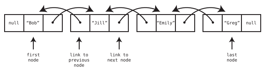
A doubly linked list is like a linked list except that each node has two links—one that points to the next node, and another that points to the previous node. In addition, the doubly linked list always keeps track of both the first and last nodes, instead of just the first node.
-
Insertion and deletion at front and back
Because doubly linked lists have immediate access to both the front and end of the list, they can insert data on either side at O(1) as well as delete data on either side at O(1).
-
Doubly linked list as queue
Because doubly linked lists can insert data at the end in O(1) time and delete data from the front in O(1) time, they make the perfect underlying data structure for a queue.
-
Chapter 15: Speeding Up All The Things With Binary Search Trees
-
Why trees?
Sorting in the best case scenario takes O(N log N) as we saw earlier. If we want a data structure that maintains order yet also has fast search, insertion, and deletion? Neither an ordered array nor a hash table is ideal. Enter the binary search tree.
-
Tree
In a classic linked list, each node contains a link that connects the node to a single other node. A tree is also a node-based data structure, but within a tree, each node can have links to multiple nodes.
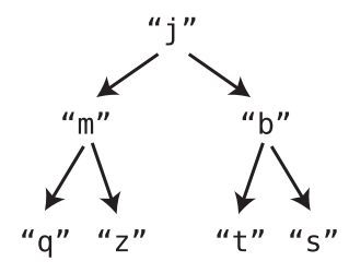
A simpler representation is shown below:
-
Balance of a tree
A tree is balanced when its nodes’ subtrees have the same number of nodes in it.
-
-
Binary Search Trees (BST)
-
Binary Tree - Each node has 0, 1 or 2 children.
-
Binary search tree is a binary tree has also has foll. rules
-
Each node can have at most one “left” child and one “right” child.
-
A node’s left descendants can only contain values lesser than the node itself. Likewise, a node’s right descendants can only contain values that are greater than the node itself.
-
-
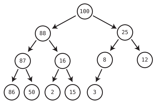
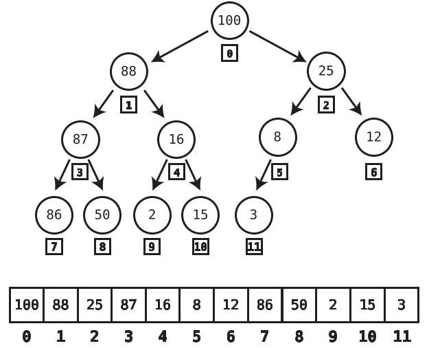
Example
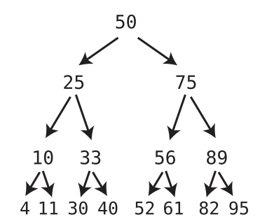
Note that each node has one child with a lesser value than itself, which is depicted using a left arrow, and one child with a greater value than itself, which is depicted using a right arrow.
Additionally, notice that all of the 50’s left descendants are less than it. At the same time, all of the 50’s right descendants are greater than it. The same pattern goes for each and every node.
-
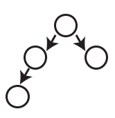
Counterexample (valid binary tree but not a binary search tree)
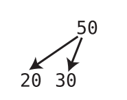
It is a valid binary tree because each node has 0, 1 or 2 children. But this is not a valid binary search tree. This is because nodes in binary search tree can have at most one left child and at most one right child, with the left child lesser than the node and the right child greater than the node.
Here, however the root has 2 left children.
-
-
Search in Binary Search Tree
-
Algorithm
Start at root. If value to be searched is lesser than root, go left. If value is more than root, go right. Repeat until we have a hit or reach bottom of the tree.
-
Efficiency of search in Binary Search Tree
-
For a perfectly balanced BST, searching is O(log N)
-
Why?
Say a BST has four complete levels. It thus has 15 nodes. When we add a fifth complete level to this BST, we add 16 new nodes. This essentially doubles the number of nodes present in the tree.
This property holds for BST. Whenever we add a new complete level, we double the number of nodes and add 1.
Each new level doubles the size of the tree. Hence, a tree containing N nodes will require log (N) levels to hold all the nodes.
This is why searching in BST takes O(log N) time: because each step of the search causes us to move down a level, we take up to as many steps as there are levels in the tree.
-
-
-
Time complexity for different operations in Ordered Array vs BST
Operation Ordered Array BST Search O(log N)
[Binary Search]O(log N)
[When tree is perfectly balanced]Insertion O(N) O(log N) Deletion O(N) O(log N) Tree traversal - O(N)
[by definition] -
Deletion
-
If the node being deleted has no children, simply delete it.
-
If the node being deleted has one child, delete the node and plug the child into the spot where the deleted node was.
-
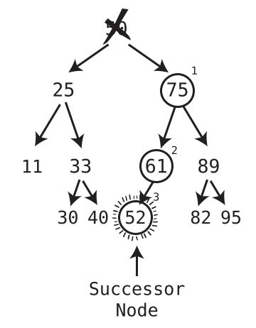
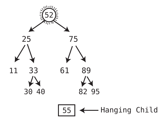
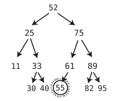
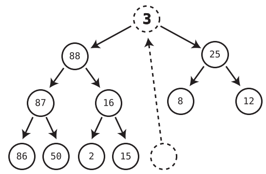
When deleting a node with two children, replace the deleted node with the successor node. The successor node is the child node whose value is the least of all values that are greater than the deleted node.
-
How to find the successor node?
Visit the right child of the deleted value, and then keep on visiting the left child of each subsequent child until there are no more left children. The bottom value is the successor node.
-
-
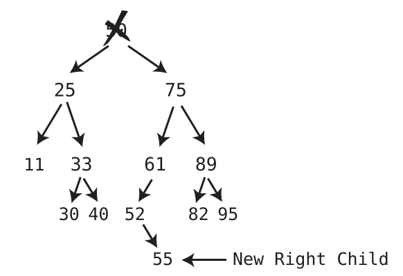
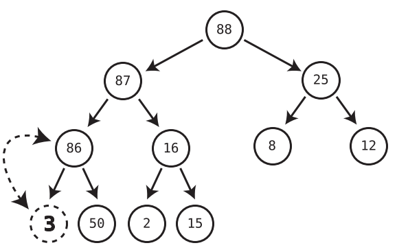
If the successor node has a right child, after plugging the successor node into the spot of the deleted node, take the former right child of the successor node and turn it into the left child of the former parent of the successor node.
-
Chapter 16: Keeping your Priorities Straight with Heap
Heap is a tree data structures that helps to constantly keep tabs on the greatest or least data element in a dataset. Before diving into Heap we understand an abstract data structure called Priority Queue. This can be implemented using other fundamental data structures.
-
Priority Queue
It is a Queue following FIFO principle i.e. access and deletion only at front of the queue. Insertion is where a traditional Queue and Priority Queue differ.
Traditional Queues insert only at the end of the Queue. Priority Queue’s insertions are like an ordered array. It inserts a new entry in a the correct spot so as to keep the Priority Queue sorted in a specific order.
Eg for priority queue: an application that manages the triage system for a hospital emergency room.
-
Implementing Priority Queue using Ordered Array
-
Deletion:
We treated the end of the ordered array as the front of the queue. Since deletions from end of array are O(1) this means access and deletions from Priority Queue are also O(1).
-
Insertion:
Inserting into an ordered array is O(N). Hence, the same applies for Priority Queues as well. Heaps serve as a more efficient foundation of Priority Queues.
-
-
Heaps
-
Heaps are a type of binary tree. Recap:
-
Binary Tree - A tree in which every node can have a maximum of two children.
-
Binary search tree is a specific type of Binary tree.
-
Heaps are also a specific type of Binary trees.
-
-
Heaps can be max-heap / min-heap.
-
Conditions for max-heaps (called heap from now on)
-
The value of each node must be greater than each of its descendant nodes. This is know as the heap condition.
-
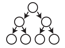
The tree must be complete.
A complete tree is a tree that is completely filled with nodes; no nodes are missing. However, the bottom row can have empty positions, as long as there aren’t any nodes to the right of these empty positions.
-
Following is a complete tree
-
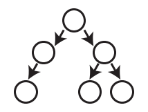
Following is an incomplete tree
-
Following is again a complete tree
-
-
-
Min-heap
Similar to max-heap but every node contains a smaller value than any of its descendants.
-
Properties of Heaps
-
Seaching values in heaps and ordering of heaps:
Heaps are weakly ordered while Binary Search Trees are strongly ordered. This is because though Heaps have a certain ordering (descendants cannot be larger than ancestors), it in no way helps while trying to search for a value within the heap. This is not the case in Binary Search Trees.
Searching for a value in Heaps requires that each node be visited. Hence, searching is not a common operation implemented in the context of Heaps.
-
Last node of Heap
Right most node in the bottom row.
-
-
Heap Insertion operation
-
Algorithm
-
Create a node containing the new value and insert it in the rightmost available spot in the bottom level. The new node thus becomes the last node of the heap.
-
Compare the new node with the parent node.
-
If the new node is greater than the parent node, we swap the new node with the parent node.
-
Repeat above step, effectively moving the new node up through the heap, until it has a parent whose value is greater than it.
-
-
But how do you find the last node position? (See below)
-
-
Heap Deletion operation
We only ever delete the root node.
-
Algorithm
-
Move the last node into where the root node was, effectively removing the original root node. (Refer below to see how to find last node)
-
Trickle the root node down into its proper place.
-
We check both children of the trickle node (former last node that is now the root node) and see which one is larger.
-
If the trickle node is smaller than the larger of the two child nodes, we swap the trickle node with that larger child.
-
We repeat Steps 1 and 2 until the trickle node has no children who are greater than it.
-
-
-
-
-
Time complexity of Heaps v/s Ordered Arrays
Ordered Arrays Heap Insertion O(N) O(log N) Deletion O(1) O(log N) Hence, heaps are the optimal choice for implementing priority queues because priority queues perform addition and deletion in equal proportions.
-
Finding last node of heap
-
Importance of last node
Insertion in heap is only permitted to take place in last node position and deletion requires last node to replace root node so that the heap is complete. A complete heap implies a balanced tree. A balanced tree is required because it is the most important characteristic that keeps time complexity to O(log N). Else, if all nodes were stacked below each other in a straight line (unbalanced tree), operations would take O(N) instead of O(log N).
-
Finding last node of heap by implementing heaps using Arrays
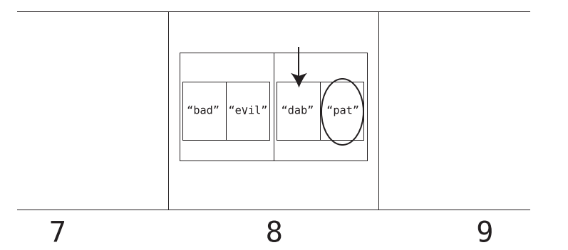
We started with wanting to implement abstract data structure Priority Queues using Heaps. But in fact, heaps themselves are abstract data structures and are implemented using Arrays. Following figure shows how heaps are transformed into arrays.
In this setup, the last node of the heap will always be the final element of the array. Additionally, when we insert a new node into the heap, we do so at the end of the array in order to make it the last node.
-
-
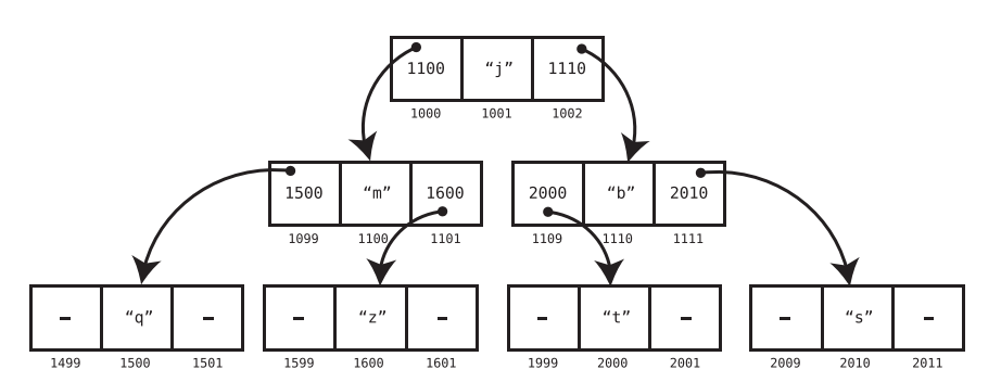
Implementing Binary Trees using Arrays
Any binary tree, not just heaps can be implemented using Arrays. This include Binary Search Trees as well. But Heaps was the first instance where implementing it using Arrays gave a marked improvement because it helped us find the last node easily.
-
Heapsort
If values are added one by one in a brand-new max-heap and then pop values from the heap one at a team and insert these values into a new array, this new array would have the numbers in descending order.
This is another sorting algorithm. Like quicksort this too take O(N logN). This is we have to insert N values and each insertion takes log N time.
Chapter 17: It Doesn’t Hurt to Trie
You have a autocomplete application on your phone. You type “catn” and the autocomplete feature suggests catnip / catnap. How does it do it so efficiently? The application needs to have access to all the dictionary words and then suggest likely words you’d be typing starting with catn.
If we had an ordered array, using binary search we can find the words in O(log N). But using the tree based data structure Trie we can get O(1) speeds.
Tries are ideal for text based features like autocomplete, autocorrect and apps involving IP addresses or phone numbers.
-
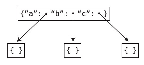
The Trie Node
The Trie is not a binary tree. In a binary tree a node can only have a maximum of 2 children. But a Trie node can have any number of child nodes.
In this implementation, each Trie node has a hash table. The keys of this hash table are English alphabets and the values point to other nodes in the Trie.
-
Tries storing words
The Trie stores words ace, act, bad, cat in the following manner:
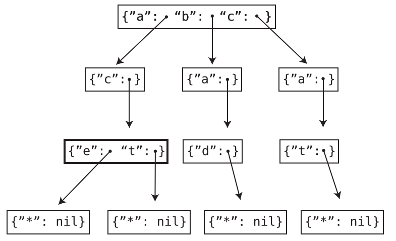
How does it store the words “bat” and “battery”?
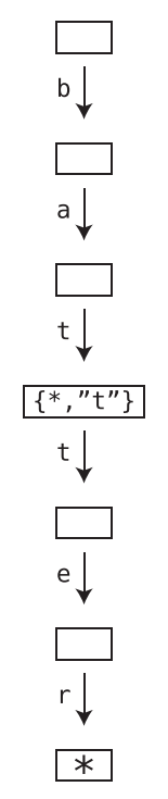
The Trie node with key “t” (for first t) has a value that points to a node with the following hash table (dict): {“”: None, “t”: *points to next t}
This indicates that bat itself is a valid word. But it also forms the prefix of another word. To access this other word following value of key “t”.
-
Efficiency of Trie Search: O(K) and not O(N)
Generally when we say an algorithm’s time complexity is \(O(N)\) or \(O(N^2)\) this refers to how the algorithm slows down wrt to the size of the data structure it deals with. For example, an increase in the size of the array will mean the algorithm slows down further.
But the case of searching in Tries is different. Irrespective of how large the Trie is, the time it takes to search a string depends on the size of the search string itself and not on the Trie.
Hence, we do not mention the efficiency of Trie search as O(N). Because this would mean as the Trie grows in size, the search slows down correspondingly.
Instead, we say search in Trie has time complexity of O(K) where K refers to the length of the search string. If the search string is of length 3, the search algorithm takes 3 steps.
We could have also used an ordered array for the autocomplete feature. Here, binary search would have taken O(log N). But here N is the length of the ordered array and recall that the ordered array contains all the words in the dictionary.
-
Efficiency of searching and insertions in Tries
Time Complexity
of TriesSearching O(K) Insertion O(K) where K is the length of the string to be searched / added.
-
Exercise: found here
Chapter 18: Connecting Everything with Graphs
-
Why Graphs?
Imagine we had a social network and we want to maintain a list of mutual friendships i.e. if A is a friend of B, then B also is a friend of A.
A basic approach is to use a 2D array to record the friendships.
But to find Alice’s friends we have to look through each subarray (each friendship). This is a O(N) algorithm.
However, using graphs we can reduce this time to O(1).
    friendships = [
        ["Alice", "Bob"],
        ["Bob", "Cynthia"],
        ["Alice", "Diana"],
        ["Bob", "Diana"],
        ["Elise", "Fred"],
        ["Diana", "Fred"],
        ["Fred", "Alice"]
]-
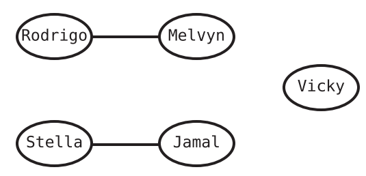
Graphs vs Trees
Trees are a subset of graphs. A graph is considered a tree when :
- It does not have cycles
- Every node is somehow connected to every other node.
The following is a graph but not a tree because Vicky node is not connected to other nodes. Also, Rodrigo is not connected to every other node and so on.
-
Graph Jargon
- Nodes -> Vertices
- Lines b/w Vertices -> Edges
- Adjacent vertices (also called neighbors) -> Vertices connected by an edge
-
Connected graph ->
Though it is possible to have a vertex in a graph that is not connected to any other vertex, a graph where all the vertices are connected in some way is called a connected graph.
Note that having a connected graph does not mean we have a tree. Connected graphs can still have cycles. Not having cycles is a prerequisite for a tree.
-
Meaning of graph search
Disclaimer: We’ll be dealing with connected graphs.
Search in a list for examples means we are looking if a specific value exists in the list.
Searching in graphs has a similar but slightly different meaning. It has following scenarios:
-
We have access to a random vertex in the graph (Alice). If search wants to find out Bob vertex, it means we need to find out if there is a path from Alice to Bob.
-
We have access to a random vertex in the graph (Alice) and we traverse all other vertices in the graph.
-
-
Efficiency of graph search: O(V + E)
The numbers of steps involved in graph traversal / search increases when we increases the number of vertices or number of edges.
Both graphs below have the same number of vertices - 5. But graph A-B-C-D-E takes 21 steps while graph V-W-X-Y-Z takes 13 steps. These steps include the 5 steps to actually traverse the vertices plus the additional steps required to iterate over the neighboring vertices.
_1.png)
_2.png)
Chapter 19: Dealing with Space Constraints
-
Big question for Big O for time complexity v/s space complexityä
Big O notation is used to represent both time and space complexity. But the key question that Big O answers differs for both:
-
Time complexity:
if there are N data elements, how many steps will the algorithm take?
-
Space complexity:
if there are N data elements, how many auxiliary units of memory will the algorithm consume?
Auxiliary here means that apart from the memory required to accommodate the input list or other data structure, how much extra memory does the function code itself create to process the input data.
This is why the following code which creates a brand new array to make list elements uppercase has space complexity of O(N) while the second code snippet which makes list elements uppercase in place has O(1) complexity.
But depending on the resource referred to, some of them also factor in the space occupied by the inputs while calculating space complexity.
 // Space complexity: O(N)
 // Time complexity: O(N)

 function makeUppercase(array) {
     let newArray = [];
     for(let i = 0; i < array.length; i++) {
         newArray[i] = array[i].toUpperCase();
     }
     return newArray;
 }
// Space complexity: O(1) // Time complexity: O(N) function makeUppercase(array) { for(let i = 0; i < array.length; i++) { array[i] = array[i].toUpperCase(); } return array; }
-
-
Space complexity in recursion
A recursive function call stores a new enter in the call stack before continuing on to the next recursion to make sure it knows where in the outer function control must return once the inner function has been successfully executed.
Every recursive call hence places a new entry in the call stack. The computer only allows a certain number of entries in the call stack.
In cases of recursion, even though there might not be a new list being created or something similar, the max number of entries in the call stack will be the space complexity.
Chapter 20: Techniques for Code Optimization
-
Incorporating blazing fast lookups using hash tables can be an effective strategy in cutting down runtime.
-
Greedy algorithms
-
Defintion:
A greedy algorithm is one that, in each step, chooses what appears to be the best option at that moment in time.
-
Example - Array Max
To find the max value in an array, we first consider array[0] to be the max_value. As we iterate through the array, when we encounter a bigger value than the current max_value, we update the max_value to this newer value.
This familiar algorithm is also an example of a greedy algorithm.
-